Intro to DirectX Raytracing: The concepts (part 1)
Computer graphics is evolving rapidly. More techniques are applied, optimizations are created and we got more computational power as ever before. Everything to make the final image look as realistic as possible (or not). In 2018, Nvidia announced their new graphics card with ‘special’ RT cores. This meant, that shipping games with ray traced and more realistic graphics was possible, all while it was smooth and enough for gamers to enjoy those beautiful graphics.
The following articles will show my interpretation on what DirectX Raytracing is and how it works. After reading these articles, you would be able to create a ray tracer using DXR, and you are able to expand it with new ray tracing concepts or resources. In a later article I will also show you how you can use inline ray tracing from different shaders to utilize the ray tracing capabilities.

Table of content
Basics
But what is ray tracing exactly? Ray tracing is a simulation of light transportation, which simulates the lighting better than the before used method for computer graphics,rasterization. The main downside, performance, as it is not a method that is really great for the architecture of the computer as we know it today. Luckily, the GPU manufacturers are pushing the boundaries of GPU performance, making sure we can use ray tracing as our method of rendering graphics, rather than it remaining in movies or other applications.
Vector Math
So, how do we trace our rays? Lets start with the basics and the most scary part for a lot of people. Math!. Do not worry. I will try to make it as simple as possible, so a trained monkey can trace rays using the math examples I will provide.
Ray tracing mainly consists of vector math. A vector consists of multiple numbers representing either a position or a direction within a coordinate system. For our case, we will have a vector of three numbers for our 3D world. Mathematicians would note a 3D vector as the following:
\[\begin{pmatrix} x \\ y \\ z \end{pmatrix}\]A ray consists of at least two vectors. One is for the direction the ray goes, and one for the origin. As last, a ray has a distance, which we call t (or lambda), that is used to determine the end position of the ray.
\[x = \vec{O} + \vec{D} * t\]\[\vec{t}_n = \dfrac{\vec{t}}{||\vec{t}||}\]Note: The direction of the ray has to be normalized (magnitude needs to be 1.0) to be to make sure we do not go through and skip our geometry. We can do that by dividing the vector by the length of the vector.
Normalizing a vector.
Lets do a simple example. Lets say, we are at the coordinate (2.5, -1.0, 0.0) and we look towards (0.5, 0.5, 0.0). At a distance of 3.0, there is an object. If we use the before mentioned formula, we can calculate the location of that object.
\[x = \vec{O} + \vec{D} * t\] \[\begin{pmatrix} x \\ y \\ z \end{pmatrix} = \begin{pmatrix} 2.5 \\ -1.0 \\ 0.0 \end{pmatrix} + \begin{pmatrix} 0.5 \\ 0.5 \\ 0.0 \end{pmatrix} \times 3.0\] \[= \begin{pmatrix} 2.5 \\ -1.0 \\ 0.0 \end{pmatrix} + \begin{pmatrix} 1.5 \\ 1.5 \\ 0.0 \end{pmatrix}\] \[= \begin{pmatrix} 4.0 \\ 0.5 \\ 0.0 \end{pmatrix}\]Now we know where the object is in the world ((4.0, 0.5, 0.0) in this case) and we can do more calculations based on that position (e.g. lighting, shadows, reflections, …). If we take that to C/C++ code it would look like this:
struct Ray
{
    float3 Origin;      // O
    float3 Direction;   // D
    float  Distance;    // t
};

float3 GetWorldPosition(const Ray& ray)
{
    return ray.Origin + ray.Direction * ray.Distance;
}
Ray Generation
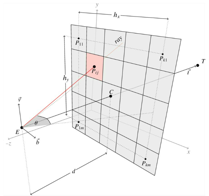
The creation, or so called ‘generation’ of the rays is very simple. A ray gets generated by having the camera’s position as the origin and the direction that goes through a pixel of the render target from the camera’s perspective. This can be one ray per pixel or more, if that is desired.
This can be done as seen below in pseudo code (HLSL equivalent by Microsoft in their sample). This takes the projection into account, so the user can change it easily by just changing the matrices.
Ray GetPrimaryRay(const float3& cameraPosition, uint2 index, const float4x4& inverseVP)
{
    Ray ray = {};
    ray.Origin = cameraPosition;

    // Set the position on the middle of the pixel
    float2 screenPos = float2(index) + float2(0.5f);

    // Transform from [0..ScreenDimension] to [0..1]
    screenPos = screenPos / RenderTargetDimensions; // we get to this later on how you get this.

    // Transform from [0..1] to [-1..1] to apply the correct projection
    screenPos = screenPos * 2.0f - 1.0f;

    // Depending on the graphics API. For DXR, it is needed...
    screenPos.y = -screenPos.y;

    // Transform from clip to world space
    float4 world = inverseVP * float4(screenPos, 0.0f, 1.0f);

    // Perspective divide
    world.xyz /= world.w;

    // Create ray direction
    ray.Direction = normalize(world.xyz - cameraPosition);

    return ray;
}
Ray Intersection
So we know where our camera is in the scene, the direction and where an object is with all its properties. But we are missing one key aspect. We do not know what the closest object is to the camera that the ray intersects with. That is where the intersection functions come into play. These functions calculate if the ray intersects with the object and at what distance. Lets start with a simple intersection function. The one from a sphere.
\[\text{$r^2 = x^2 + y^2 + z^2,\:$ where $\:r^2 < x^2 + y^2 + z^2 \:$ is inside of the sphere}\]After rewriting the function to something more useful for us (what Peter Shirley did in Ray tracing in one weekend), you would get a mathematical function that looks like this:
\[D\cdot D \times t^2 - 2 \times t \times D \cdot (C - O) + (C - O) \cdot (C - O) - r^2 = 0\]\(D\) is the ray direction, \(O\) is the ray origin, \(C\) is the center of the sphere and \(r\) is the radius of the sphere. The only variable that is unknown and is what we are solving for is \(t\) (the ray distance). After filling the parameters inside of this function, it looks like a quadratic equation, which can easily be solved using the so called ‘quadratic formula’.
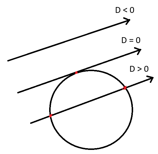
\[\frac{-b \pm \sqrt{b^2 - 4 \times a \times c}}{2 \times a}\]Lets look at the discriminant of the quadratic equation. Because there is a possibility of early out there where we can save some resources. If the discriminant is less than zero, then the ray missed the sphere entirely, making solving for \(t\) unnecessary. If the discriminant is zero or greater than zero, we have a hit and we can proceed doing all the calculations needed to solve for \(t\). Since we want the closest object to the origin, we only solve for \(t\) using the minus version of the quadratic formula.
Acceleration Structures
When ray tracing, we are using more than a couple of intersection tests. One for every triangle or primitive in the scene, making rendering an entire scene really performance intensive. An acceleration structure is a common approach to reduce the amount of intersection tests that were not needed in the first place. An acceleration structure is a data structure designed to improve application speed.
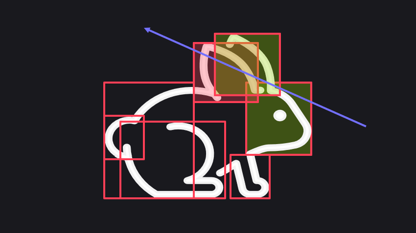
With ray tracing, we use a so called BVH or a bounding volume hierarchy. This data structure splits the scene and geometry into bounding boxes and creates a tree of those bounding boxes. It will do an AABB intersection test to check if it hit the bounding box that contains the entire tree. If it hits the tree, it will traverse the tree until it hits a leaf node (end of the tree) and return the value the renderer requests (e.g. material, vertex data, or just the colour). If it misses the root bounding box, it only did one intersection test, thus saving a lot of time.
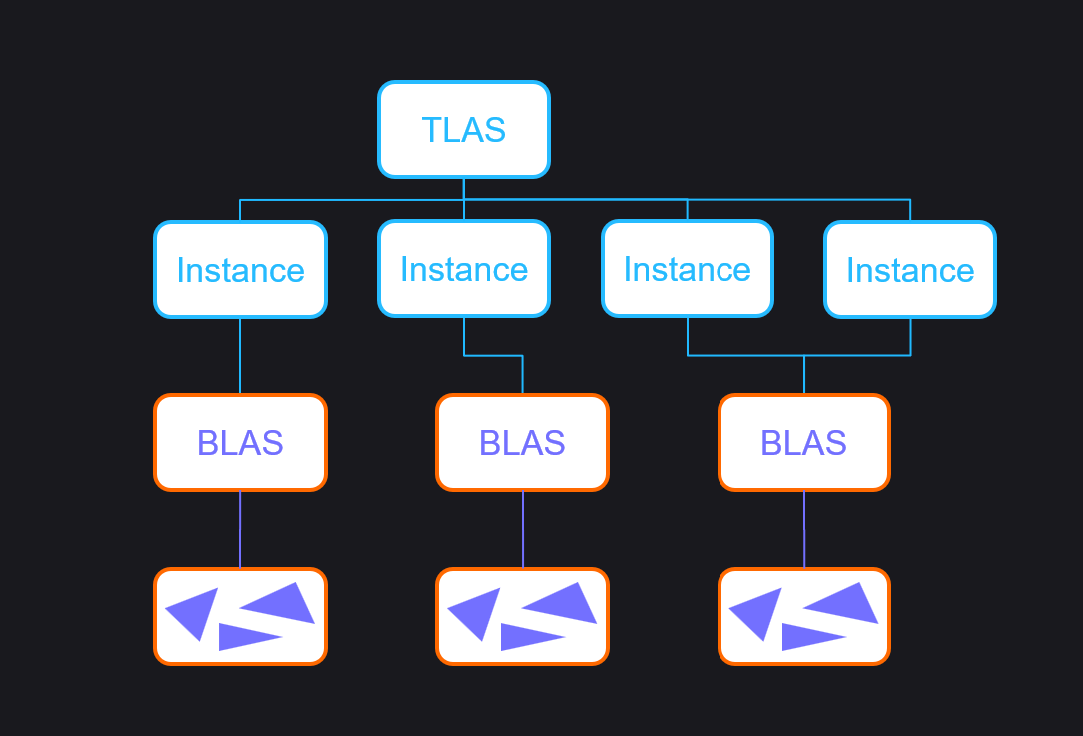
People split the accelerating structures in two parts. The BLAS (bottom level acceleration structure) and the TLAS (top level accelerating structure). The BLAS contains the geometry data (e.g. triangles and other primitives) and the TLAS contains the instance data, which contains the BLAS data. The reason for this structure, is to save on memory usage. The instances share the same acceleration structure and geometry data, making the extra geometry unnecessary. The only exception could be animated meshes.
So this is ray tracing in a nutshell. We create rays from the camera, we trace them, test them against objects and return the colour closest object to the camera to create a render target, which we present to the screen.
If you want to know more about vectors and vector math, you can watch this YouTube video from FloatyMonkey to fully understand vector math. If you want to explore more of the basics of ray tracing, check out Ray tracing in one weekend by Peter Shirley to learn more! On how to build BVHs, the article series from Jacco Bikker will explain everything to create BVHs on CPU (How to build a BVH).
DirectX Raytracing: API
Acceleration Structures in DXR
Shaders
With this API, comes a new set of shaders. As ray tracing replaces rasterization, we will have to say goodbye to our old vertex, pixel, and other shaders, and we will bring new shaders to replace them and to do our job. Unlike the rasterization and compute shaders, these shaders are compiled as a library, rather than e.g. a vertex shader. More on that, in the next part. These are the ray tracing shaders:
Ray Generation Shader
The ray generation shader is the start of the pipeline. This shader allows you to create the rays that will be traced with your set settings. After you have ‘generated’ your ray, you trace the ray, which traverses the BVH and call the other shaders internally. The main attributes you need to have for this shader is a TLAS, an unordered access view as a 2D texture and optionally camera data.
RaytracingAccelerationStructure g_TLAS : register(t0);
ConstantBuffer<Camera> g_Camera : register(b0);
RWTexture2D<float4> g_RenderTarget : register(u0);
Because you can generate the rays yourself, you can do way more than just rendering to the render target.
struct RayPayload
{
    float4 Color;
};

[shader("raygeneration")]
void RayGenMain()
{
    float2 screenPos = float2(index) + 0.5f.xx;
    screenPos = screenPos / (float2)DispatchRaysDimensions();
    screenPos = mad(screenPos, 2.0f, -1.0f);
    screenPos.y = -screenPos.y;

    float4 direction = mul(InverseViewProjection, float4(screenPos, 0.0f, 1.0f));
    direction.xyz /= direction.w;

    RayDesc ray;
    ray.Origin = g_Camera.Position;
    ray.Direction = normalize(direction - g_Camera.Position);
    ray.TMin = 0.01f;
    ray.TMax = 1000.0f;

    RayPayload payload = { float4(0, 0, 0, 0) };

    TraceRay(g_TLAS, RAY_FLAG_CULL_BACK_FACING_TRIANGLES, ~0, 0, 1, 0, ray, payload);

    g_RenderTarget[DispatchRaysIndex().xy] = payload.Color;
}
Closest Hit Shader
The closest hit shader is the shader that gets run for the closest instance in the scene. This is the final step in the TraceRay() sequence, if the ray intersects with an instance. In this shader, you can set the ray pay load of the ray. This can be the shading of the pixel, or passing any data you can think of.
There are some useful helper functions that are available in the closest hit shader that you need to be aware of:
float3x4 ObjectToWorld3x4()/ float4x3 ObjectToWorld4x3(): The matrix that transforms the vertex data from object space to world space. Two variants exist for the matrix orientation some might use (transpose of the matrix will get the other matrix).float3x4 WorldToObject3x4()/ float4x3 WorldToObject4x3(): The matrix that transforms the vertex data from world space to object space (inverse ofObjectToWorld3x4()/ObjectToWorld4x3()).
float3 WorldRayOrigin(): The origin of the ray in world space.float3 ObjectRayOrigin(): The origin of the ray in object space. Object space is the space of the current BLAS.
float3 WorldRayDirection(): The direction of the ray in world space.float3 ObjectRayDirection(): The direction of the ray in object space. Object space is the space of the current BLAS.
float TMin(): The start distance of the ray.float TCurrent(): The distance of the ray where the closest hit occurred.
uint InstanceID(): Returns the ID of the instance set in the TLAS.uint InstanceIndex(): Returns the autogenerated index of the instance in the TLAS.uint PrimitiveIndex(): Returns the autogenerated index of the primitive in the BLAS.
All of these functions are available for the closest hit, any hit, intersection and miss shader. Only the last three functions are not available in the miss shader. This is because the ray missed all the possible instances, meaning that that data is not present.
// This example uses bindless rendering from shader model 6.6. Default binding is also possible.

struct RayPayload
{
    float4 Color;
};

struct Mesh
{
    float4 Color;

    uint IndexIdx;
    uint NormalIdx;
    uint UV0Idx;
};

StructuredBuffer<Mesh> g_ModelData : register(t0);

[shader("closesthit")]
void ClosestHitMain(inout RayPayload payload, in BuiltInTriangleIntersectionAttributes attr)
{
    float3 barycentrics = float3(1 - attr.barycentrics.x - attr.barycentrics.y, attr.barycentrics.x, attr.barycentrics.y);
    Mesh model = g_ModelData[InstanceID()];

    ByteAddressBuffer indexBuffer = ResourceDescriptorHeap[model.IndexIdx];
    StructuredBuffer<float3> normalBuffer = ResourceDescriptorHeap[model.NormalIdx];

    uint3 indices = indexBuffer.Load3(PrimitiveIndex() * 3 * 4 /*sizeof(uint)*/); // assume we have 32-bit indices

    float3 normal0 = normalBuffer[indices.x] * barycentrics.x;
    float3 normal1 = normalBuffer[indices.y] * barycentrics.y;
    float3 normal2 = normalBuffer[indices.z] * barycentrics.z;

    float3 normal = normalize(normal0 + normal1 + normal2);
    normal = mul((float3x3)ObjectToWorld3x4(), normal);

    payload.Color = float4(mad(normal, 0.5f, 0.5f), 1.0f);
}
This shader can call TraceRay(). This would be useful if we want to cast a shadow ray, reflection ray or a different ray for extra data input. If needed, use a different shader from the shader table and different flags to make it the most optimal. As this can introduce a lot of recursion, you can set the max recursion in the pipeline and/or use a safe guard to prevent infinite loops.
struct RayPayload
{
    float4 Color;
    uint Depth;
};

[shader("closesthit")]
void ClosestHitMain(inout RayPayload payload, in BuiltInTriangleIntersectionAttributes attr)
{
    if (++payload.Depth >= MAX_RECURSION)
    {
        payload.Color = 1.0f.xxxx;
        return;
    }

    float3 barycentrics = float3(1 - attr.barycentrics.x - attr.barycentrics.y, attr.barycentrics.x, attr.barycentrics.y);
    Mesh model = g_ModelData[InstanceID()];

    ByteAddressBuffer indexBuffer = ResourceDescriptorHeap[model.IndexIdx];
    StructuredBuffer<float3> normalBuffer = ResourceDescriptorHeap[model.NormalIdx];

    uint3 indices = indexBuffer.Load3(PrimitiveIndex() * 3 * 4 /*sizeof(uint)*/); // assume we have 32-bit indices

    float3 normal0 = normalBuffer[indices.x] * barycentrics.x;
    float3 normal1 = normalBuffer[indices.y] * barycentrics.y;
    float3 normal2 = normalBuffer[indices.z] * barycentrics.z;

    float3 normal = normalize(normal0 + normal1 + normal2);
    normal = mul((float3x3)ObjectToWorld3x4(), normal);

    RayPayload newPayload = { float4(0.0f.xxxx); payload.Depth };

    RayDesc ray;
    ray.Origin = WorldRayOrigin() + WorldRayDirection() * TCurrent();
    ray.Direction = reflect(WorldRayDirection(), normal);
    ray.TMin = 0.01f;
    ray.TMax = 1000.0f;

    TraceRay(g_TLAS, RAY_FLAG_CULL_BACK_FACING_TRIANGLES, ~0, 0, 1, 0, ray, newPayload);

    payload.Color = float4(normal + newPayload.Color, 1.0f);
}
Any Hit Shader
The any hit shader is similar to the closest hit shader. The main difference is, is that this shader does not result per se in the end of the TraceRay() sequence. The geometry that goes through this shader, is marked as transparent, which allows us to add transparency to pipeline.
You can also do some blending using the colour output on the payload. But in my opinion, tracing a ray that is refracted would be better, for more realistic results.
The any hit shader gets two functions to control the flow of the traversal.
IgnoreHit(): Ignore the hit and end the shader. The traversal will continue as if nothing was in the way.AcceptHitAndEndSearch(): Accept the hit and end the shader. The TMax and the attributes will be set and the traversal will stop, resulting of the invocation of the closest hit shader.
If we want to accept the hit and continue the traversal, we can just end the code block of the shader. That way, the TMax will update, but it will continue.
// This example uses bindless rendering from shader model 6.6. Default binding is also possible.

struct Mesh
{
    uint AlbedoIdx;

    uint IndexIdx;
    uint NormalIdx;
    uint UV0Idx;
};

StructuredBuffer<Mesh> g_ModelData : register(t0);
SamplerState g_Sampler : register(s0);

[shader("anyhit")]
void AnyHitMain(inout RayPayload payload, in BuiltInTriangleIntersectionAttributes attr)
{
    float3 barycentrics = float3(1 - attr.barycentrics.x - attr.barycentrics.y, attr.barycentrics.x, attr.barycentrics.y);
    Mesh model = g_ModelData[InstanceID()];

    ByteAddressBuffer indexBuffer = ResourceDescriptorHeap[model.IndexIdx];
    StructuredBuffer<float2> uv0Buffer = ResourceDescriptorHeap[model.UV0Idx];

    uint3 indices = indexBuffer.Load3(PrimitiveIndex() * 3 * 4 /*sizeof(uint)*/); // assume we have 32-bit indices

    float2 uv0 = uv0Buffer[indices.x] * barycentrics.x;
    float2 uv1 = uv0Buffer[indices.y] * barycentrics.y;
    float2 uv2 = uv0Buffer[indices.z] * barycentrics.z;

    float2 uv = uv0 + uv1 + uv2;

    Texture2D<float4> Albedo = ResourceDescriptorHeap[model.AlbedoIdx];
    float4 albedoSample = Albedo.SampleLevel(Sampler, uv, 0);

    if (albedo.a < 0.1f)
    {
        IgnoreHit();
    }
}
Miss Shader
The miss shader gets run when there is no instance that intersects with the ray. Same as the closest hit shader, this the end of the TraceRay() sequence. This shader can be used to sample the sky dome, or can be used for a variety of purposes. Take shadow rays as an example (see second example).
// This example uses bindless rendering from shader model 6.6. Default binding is also possible.

struct RayPayload
{
    float4 Color;
};

struct Scene
{
    uint SkydomeIdx;
}

ConstantBuffer<Scene> g_Scene : register(b0);
SamplerState g_Sampler : register(s0);

[shader("miss")]
void MissMain(inout RayPayload payload)
{
    TextureCube<float4> skydome = ResourceDescriptorHeap[g_Scene.SkydomeIdx];

    payload.Color = float4(skydome.SampleLevel(g_Sampler, WorldRayDirection(), 0).rgb, 1.0f); // ignore the alpha channel
}
struct RayShadowPayload
{
    bool IsOccluded;
};

[shader("miss")]
void ShadowMissMain(inout RayShadowPayload payload)
{
    payload.IsOccluded = false;
}
Intersection Shader
When the ray hits an instance, it could be a triangle. The triangle intersection is a fixed function, so no flexibility is there. The intersection shader allows you to add intersection tests to the ray traversal for primitives that are not triangles. In this shader, you can report a hit if the primitive was hit according to your rules.
To indicate that a ray hit the procedural primitive, ReportHit() needs to be called in the intersection shader. Pass the t value of the ray, the hit kind, and the attributes to the ReportHit() function to report a hit. If ReportHit() does not get called, a miss is assumed and the ray traversal will continue.
struct PrimitiveAttributes
{
    float3 Normal;
};

[shader("intersection")]
void IntersectionMain()
{

    // https://raytracing.github.io/books/RayTracingInOneWeekend.html#addingasphere/ray-sphereintersection
    float3 position = 1.5f.xxx;
    float radius = 0.5f;

    float3 oc = position - WorldRayOrigin();
    float a = dot(WorldRayDirection(), WorldRayDirection());
    float h = dot(WorldRayDirection(), oc);
    float c = dot(oc, oc) - radius * radius;
    float discriminant = h * h - a * c;

    if (discriminant >= 0.0f)
    {
        PrimitiveAttributes attr;
        attr.Normal = 1.0f.xxx;

        float t = (h - sqrt(discriminant)) / a;
        float3 normal = normalize((WorldRayDirection() * t + WorldRayOrigin()) - position);

        ReportHit(t, 0, attr);
    }
}
Raytracing Pipeline
The ray tracing pipeline is a bit different than the older rasterization pipeline. Instead of going from shader A to shader B, this pipeline has a complex and modular flow, as can be seen below.
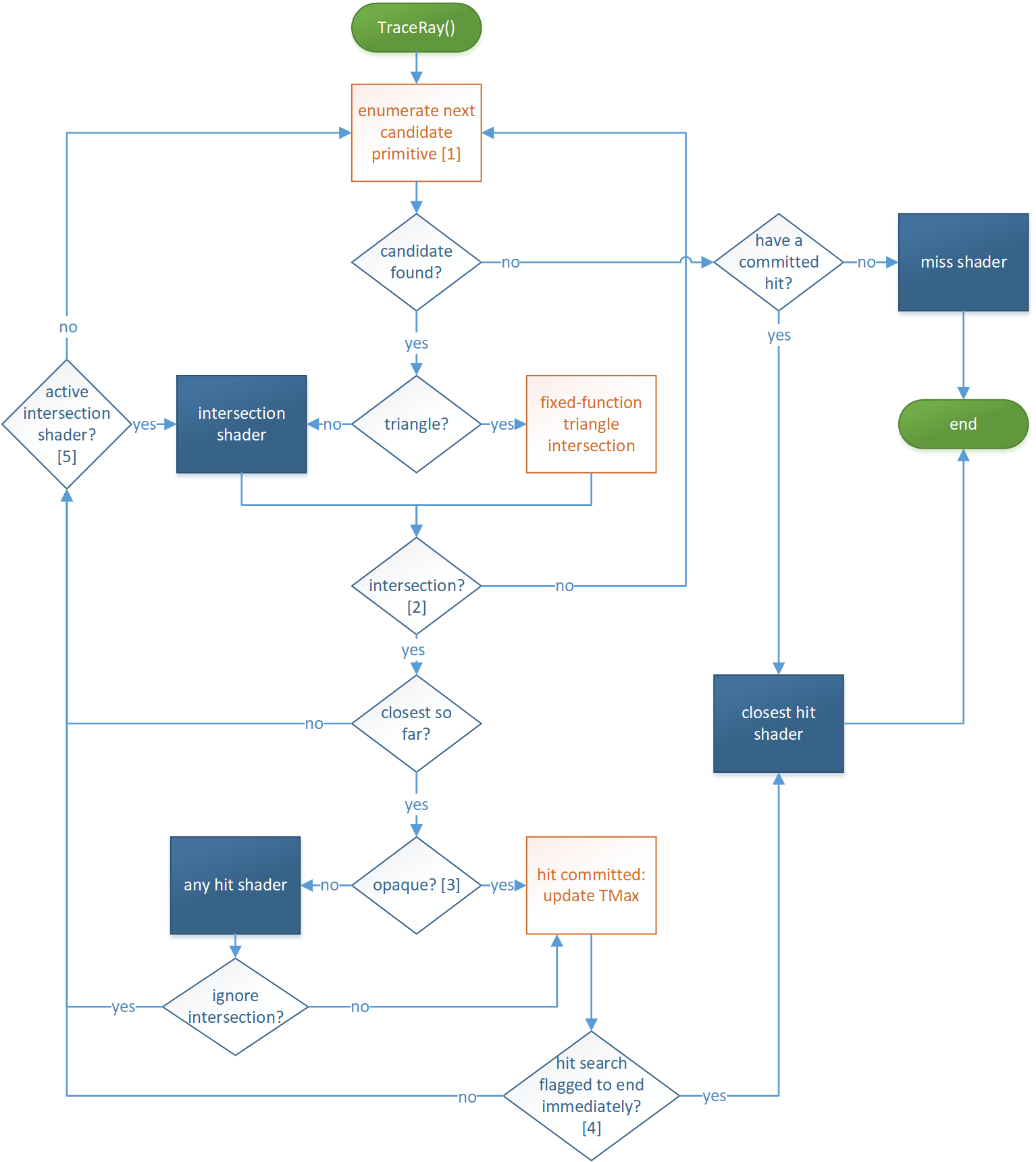
As you can see, it is a lot of information to get at first, so lets break it down.
We start with the ray generation shader. There we generate the ray and call the TraceRay() function. This function starts the entire pipeline, as seen at the top of the pipeline overview.
Intersection
The ray starts traversing the acceleration structure, where it checks if it can find instances along the ray. If the ray finds an instance, the pipeline checks if it is a triangle or if it is a AABB. If it is an AABB, our intersection shader will be ran to test if the ray intersects. If the ray do not intersect with an instance, it traverses further, until it hits something or if it is at the end of the acceleration structure, which will result in a miss.
Hit
The ray hit an instance, what is next? The instance gets checked, if it is opaque or transparent. If the instance is transparent, the any hit shader evaluates if we need to ignore the hit, because the object is transparent. The ray will traverse further. It the instance is ‘tinted’, the hit will be ignored, but the colour of the object will be passed to the payload. Else the hit will be treated as an opaque hit.
Hit Groups
So how do we tie everything together, and do I have to use multiple pipelines if I want to use the multiple primitives in my raytracer? The hit groups answer that question. A hit group is a group of shaders that are invoked on hits. These shaders are an intersection shader, an any hit shader and a closest hit shader. But how do you determine which hit group is associated with which instance? You pass it when creating the instance. in the struct D3D12_RAYTRACING_INSTANCE_DESC, there is a variable called ‘’ where you can specify the hit group index for that specific instance.
Optimizations
To speed up the ray traversal process, we can cut some corners here and there (depending on the case we have). When we call TraceRay(), we can pass flags to it. These flags are the following:
enum RAY_FLAG : uint
{
    RAY_FLAG_NONE = 0x00,
    RAY_FLAG_FORCE_OPAQUE = 0x01,
    RAY_FLAG_FORCE_NON_OPAQUE = 0x02,
    RAY_FLAG_ACCEPT_FIRST_HIT_AND_END_SEARCH = 0x04,
    RAY_FLAG_SKIP_CLOSEST_HIT_SHADER = 0x08,
    RAY_FLAG_CULL_BACK_FACING_TRIANGLES = 0x10,
    RAY_FLAG_CULL_FRONT_FACING_TRIANGLES = 0x20,
    RAY_FLAG_CULL_OPAQUE = 0x40,
    RAY_FLAG_CULL_NON_OPAQUE = 0x80,
    RAY_FLAG_SKIP_TRIANGLES = 0x100,
    RAY_FLAG_SKIP_PROCEDURAL_PRIMITIVES = 0x200,
    RAY_FLAG_FORCE_OMM_2_STATE = 0x400,
};
These ray flags are self explanatory on what they do and as you can see, some evaluation steps can be removed, if we do not use those parts of the pipeline at all.
Also a thing to note, the intersection shader and the any hit shaders are quite costly. Not because they contain code that is heavy, but because these operations run on the programmable part of the GPU, while the traversing and triangle intersection happen near the texture units of the core. This means that the intersection shader and the any hit shader execution happens quite far away in distance, costing time. The GPU vendors recommend you to refrain from using these shaders for performance reasons, if possible.
A while ago, Nvidia introduced a new way of having transparent geometry. Opacity micro maps. Opacity normally gets evaluated in the any hit shader. Since that shader gets run on the programmable part of the GPU, it can take quite some time to render the scene. Especially foliage makes great use of opacity to save triangles. So, we can use more triangles instead? No that tanks the performance. The good solution would still be the any hit shader (and profile the difference). But the best option would be the opacity micro maps. It is a map that says if a part of the geometry is opaque, transparent or if it needs to be manually tested. This eliminates the programmable implementation that needs to be created, to a more optimized version in the driver. Which means, more performance! ……if we believe Nvidia. I myself have not tried it out, as the option for DirectX Raytracing is still in preview, and will not be seen in production as of now.
Inline Raytracing
What if the entire pipeline thing is too much. We do not want this complex structure of different shaders. We can get rid of them by using inline raytracing. Inline raytracing is raytracing as you would do with the pipeline, but then using no raytracing shaders. You can just trace the rays in a compute shader. The main difference is how the shaders are ‘connected’. Normally, you would have a hit group with at least a closest hit shader and/or a miss shader. With inline raytracing, you just call the TraceRayInline() function using a ray query and the tracing of rays happens automatically. But instead of invoking the raytracing shaders, the query will return the data, on which you can respond, and simulate the raytracing shaders.
[numthreads(8, 8, 1)]
void main(uint2 dispatchThreadId : SV_DispatchThreadID)
{
    float2 screenPos = float2(index) + 0.5f.xx;
    screenPos = screenPos / (float2)dispatchThreadId;
    screenPos = mad(screenPos, 2.0f, -1.0f);
    screenPos.y = -screenPos.y;

    float4 direction = mul(InverseViewProjection, float4(screenPos, 0.0f, 1.0f));
    direction.xyz /= direction.w;

    RayQuery<RAY_FLAG_NONE> rq;

    RayDesc ray;
    ray.Origin = g_Camera.Position;
    ray.Direction = normalize(direction - g_Camera.Position);
    ray.TMin = 0.01f;
    ray.TMax = 1000.0f;

    rq.TraceRayInline(
        TLAS,
        RAY_FLAG_NONE,
        0xFF,
        ray
    );

    // Ray traversal
    while (rq.Proceed())
    {
        if (rq.CandidateType() == CANDIDATE_NON_OPAQUE_TRIANGLE)
        {
            rq.CommitNonOpaqueTriangleHit();
        }
    }

    if (rq.CommittedStatus() == COMMITTED_NOTHING)
    {
        // miss
    }
    else
    {
        // closest hit
    }
}
In the next part, I will go over how you can implement the raytracing pipelines. The codebase I will refer to can be found here.
References
- [1] Ray Tracing In One Weekend, Peter Shirley, 2018
- [2] BVH Building, Jacco Bikker, 2022
- [3] DirectX Specs, Microsoft, 2017
- [4] DirectX Samples, Microsoft